Exploring the Relationship between Number of Features and Training Time with XgBoost

As data grows in volume and complexity, understanding the intricacies of our algorithms becomes not just a matter of academic interest, but a practical necessity. XGBoost (Extreme Gradient Boosting) has gained immense popularity in the machine learning community for its performance, flexibility and horizontal scalability. XGBoost is often the go-to choice for both competition enthusiasts and industry professionals. But like any tool, its efficiency can be influenced by how well we understand it.

One of the pivotal aspects that can impact the training time of a machine learning model is the number of features it has to process. Intuitively, more features should more complexity and potentially longer training times.

In this post, we'll explore the relationship between the number of features in a dataset and the time it takes for XGBoost to train on it. Through systematic experimentation and analysis, we aim to provide insights that can guide data scientists in their feature engineering endeavors and help strike a balance between model accuracy and efficiency.

About XGBoost

XGBoost (Extreme Gradient Boosting) has gained immense popularity in the machine learning community, and there are several reasons for its effectiveness and widespread adoption:

• Performance:

  • Accuracy: XGBoost often delivers highly accurate results, outperforming other algorithms on a variety of benchmark datasets. Its ensemble nature, which involves building multiple decision trees and combining their outputs, allows it to capture complex patterns in data.

  • Speed: XGBoost is optimized for performance. It features parallel and distributed computing, making it faster than many other implementations of gradient boosting.

• Flexibility:

  • XGBoost can be used for both regression and classification tasks. It also supports ranking and user-defined prediction problems.

  • It can handle binary, multiclass classification, regression, and ranking tasks.

• Regularization:

  • One of the features that sets XGBoost apart from other boosting algorithms is its built-in L1 (Lasso regression) and L2 (Ridge regression) regularization. This helps prevent overfitting and can lead to better overall performance.

• Handling Missing Data:

  • XGBoost can automatically handle missing values during training, which can be a significant advantage over other algorithms that require explicit missing data imputation.

• Tree Pruning:

  • Unlike other gradient boosting methods that grow trees depth-wise, XGBoost grows trees depth-first and prunes them using the max_depth parameter. This depth-first approach can lead to more optimal trees.

• Cross-validation:

  • XGBoost has an efficient implementation of k-fold cross-validation, which can be used for model tuning and to prevent overfitting.

• Built-in Feature Importance:

  • XGBoost provides a straightforward way to visualize the importance of features in the model, aiding in feature selection and understanding the model's behavior.

• Scalability and Portability:

  • XGBoost is designed to be scalable and can be run on Hadoop, SGE, MPI, and other distributed environments. It's also portable and can be run on Linux, Windows, and macOS.

• Community and Development

  • XGBoost has a strong open-source community, which means regular updates, a plethora of resources, and quick bug fixes. Its popularity in machine learning competitions like Kaggle has also contributed to its widespread recognition and adoption.

• GPU Support:

  • XGBoost supports GPU acceleration, which can significantly speed up computations, especially for large datasets.

The combination of high performance, flexibility, and a range of features tailored to real-world machine learning challenges has made XGBoost a preferred choice for many data scientists and researchers. Its consistent performance in competitions and real-world applications has further solidified its reputation in the machine learning community.

The Role of Features in Machine Learning

In the simplest terms, a feature is an individual measurable property or characteristic of a phenomenon being observed. In the context of a dataset, features are often synonymous with columns or attributes. For instance, in a dataset about houses, features might include the number of bedrooms, square footage, type of flooring, and so on.

The Role of Features in Predictive Modeling

1. Representation of Data: Features are the building blocks of your dataset. They represent the dimensions of the data you're analyzing and provide the information that a machine learning model will learn from.

2. Influence on Model Accuracy: The quality and relevance of features directly impact the predictive power of a model. Good features can lead to accurate and insightful models, while irrelevant or redundant features can hinder performance.

3. Feature Engineering: This is the process of creating new features or modifying existing ones to improve model performance. It's an art as much as it's a science, and it underscores the importance of domain knowledge in machine learning.

Number of Features vs. Model Complexity

While it might be tempting to think that more features will always lead to a better model, this isn't necessarily the case. The relationship between the number of features and model performance is intricate:

1. Model Complexity: As the number of features increases, the complexity of the model generally rises. A more complex model can capture intricate patterns in the data, which might be beneficial for accuracy. However, there's a catch.

2. Risk of Overfitting: Overfitting occurs when a model learns the training data too closely, including its noise and outliers. Such a model performs well on the training data but poorly on new, unseen data. The more features you have, especially if they're not informative or if there's a lot of noise, the higher the risk of overfitting.

3. Diminishing Returns: After a certain point, adding more features might not lead to any significant improvement in model performance. Instead, it might just add to the computational cost and complexity.

4. Curse of Dimensionality: In high-dimensional spaces (i.e., with a large number of features), data becomes sparse. This sparsity makes it challenging for algorithms to find patterns and can degrade model performance.

Number of Features vs. Training Time

The relationship between the number of features and model training time is intuitive given an understand of the xgboost algorithm. The goal of this substack is to present the initial hypothesis and then test the assumptions using a set of experiments over synthetic feature sets.

Let's delve into the relationship between the number of features and training time in XGBoost, and how various hyperparameters might influence this relationship.

Intuition: Number of Features vs. Training Time

At its core, the relationship is straightforward: more features mean more data for the algorithm to process. Each additional feature introduces a new dimension of data, which increases the computational load. When XGBoost evaluates potential splits for a tree node, it must consider each feature. More features mean more potential splits to evaluate, leading to longer training times.

1. Memory Usage:

   • More features increase the memory footprint of the dataset. If the dataset becomes too large to fit into memory, it can lead to inefficiencies like swapping, which can slow down training.

2. Tree Complexity:

   • More features can lead to trees with greater depth or more branches, especially if those features are informative. Deeper and more complex trees take longer to build.

XGBoost Hyperparameters Influencing the Relationship:

In practice when working with xgboost on large datasets, xgboost hyperparameters are optimized based on the needs for model accuracy vs. training time. In this substack, we aim to understand the sensitivity of training time to xgboost hyperparameters that impact model accuracy . The following hyperparameters are considered in the experiments that follow:

1. tree_method:

   • The method used for building trees can influence training time. For instance, the hist and gpu_hist methods, which use histogram-based techniques, can be faster than the traditional exact method, especially with a large number of features. We limit experiments to ‘hist’ and ‘gpu_hist’ for this experiment.

2. max_depth:

   • This parameter sets the maximum depth of a tree. A smaller max_depth can limit the complexity of the trees and potentially speed up training, especially when there are many features.

3. colsample_bytree and colsample_bylevel:

   • These parameters control the fraction of features that are randomly sampled for building trees. By subsetting the features, you can reduce the computational load and speed up training.

4. subsample:

   • This parameter controls the fraction of the training data that's randomly sampled during each boosting round. While it's more about the number of rows than features, reducing the data size can indirectly speed up training when there are many features.

5. min_child_weight:

   • This parameter adds regularization to the tree-building process. A higher value makes the algorithm more conservative, potentially resulting in simpler trees that are faster to build.

6. alpha (Lasso regularization) and lambda (Ridge regularization):

   • Regularization can influence tree complexity. By adding penalties, the algorithm might opt for simpler trees, which can be faster to train

Setting Up the Experiment

This experiment uses synthetic datasets generated using the `make_regression` method in the sklearn machine learning package. Using synthetic data offers several advantages in the context of machine learning experimentation:

1. Control Over Data Characteristics: With synthetic data, you have complete control over various dataset characteristics, such as the number of samples, number of features, noise level, and more. This allows for systematic experimentation where you can isolate and study the impact of specific data attributes on model performance.

2. Understanding Algorithms: Synthetic datasets are invaluable when trying to understand the behavior of algorithms. For instance, by generating data with known underlying patterns or relationships, you can see if an algorithm can successfully capture those patterns.

3. Benchmarking and Comparisons: Synthetic datasets provide a consistent basis for comparing different algorithms or variations of an algorithm. Since the data remains consistent across experiments, any differences in outcomes can be attributed to the algorithms themselves.

4. Overfitting Demonstrations: By deliberately creating datasets with noise or irrelevant features, you can demonstrate the concept of overfitting. It's easier to illustrate how models can mistakenly capture noise using controlled synthetic data.

5. Handling Imbalanced Data: As discussed previously, synthetic data can be manipulated to create imbalanced datasets. This is useful for testing and developing strategies to handle class imbalance in classification tasks.

6. Reproducibility: Research and experiments using synthetic data are easily reproducible by others. Since the data generation process is deterministic and can be shared, other researchers or practitioners can recreate the exact same dataset to validate findings.

While synthetic data offers many advantages, it's essential to remember that real-world data often contains complexities, nuances, and patterns that synthetic data might not capture. Therefore, after initial experiments with synthetic data, it's crucial to validate findings and models on real-world datasets to ensure their practical applicability.

In this experiment, we use make_regression to generate synthetic datasets with varying numbers of features and for consistency, keep the number of samples constant at 1M rows. We test using 10, 50, 100, 1000, 2000, 5000, 10000 and 20000 features on a single Nvidia A10 GPU with 23GB memory. We test the full set of features over the following set of hyperparameters to vary during the experiment:

• learning_rate: [0.01, 0.1, 0.3]

• max_depth: [3, 6, 12]

• subsample: [0.5, 0.8, 1.0]

• colsample_bytree: [0.5, 0.8, 1.0]

Setting up the Environment

The experiments were run using Lambda Cloud. With Lambda GPU Cloud, we are provided with the prerequisites needed to perform reproducible research in machine learning:

• TensorFlow, PyTorch®, and all required drivers installed.

• persistent storage to save datasets, experiment results and experiment code

• root access to your instances via SSH and access via JupyterLab notebooks.

In a Jupyter Notebook hosted by Lambda, enter the following to install experiment prerequisites:

!pip install xgboost scikit-learn matplotlib py3nvml

You will need the following imports to your notebook.

import numpy as np
import time
from xgboost import XGBRegressor
from sklearn.datasets import make_regression
import matplotlib.pyplot as plt
import py3nvml.py3nvml as nvml
%matplotlib inline

The pynvml library provides programmatic access to query the utilization and memory allocation on the GPU. The following function is used to collect this data:

def get_gpu_info_nvml():
    nvml.nvmlInit()
    device_count = nvml.nvmlDeviceGetCount()
    for i in range(device_count):
        handle = nvml.nvmlDeviceGetHandleByIndex(i)
        util = nvml.nvmlDeviceGetUtilizationRates(handle)
        memory = nvml.nvmlDeviceGetMemoryInfo(handle)
        print(f"GPU ID: {i}, 
              GPU Utilization: {util.gpu}%, Memory Used:              {memory.used/1024**2:.2f}MB")
    nvml.nvmlShutdown()

The function below is used to generate synthetic data and traing a model on the data. The function returns the total time spent in training.

def benchmark_xgboost(num_features, 
                      n_samples=10000,
                      tree_method='hist',
                      learning_rate=0.1,
                      max_depth=12,
                      subsample=0.8,
                      colsample_bytree=0.8):
    X, y = make_regression(n_samples=n_samples, 
                           n_features=num_features, 
                           noise=0.1)
    
    # Initialize XGBoost regressor
    model = XGBRegressor(tree_method=tree_method,
                         learning_rate=learning_rate,
                         max_depth=max_depth,
                         subsample=subsample,
                         colsample_bytree = colsample_bytree)
    
    # Measure training time
    start_time = time.time()
    model.fit(X, y)
    return time.time() - start_time

Running the Experiments

The experiments are run from the Jupyter notebook using the following code:

feature_sizes = [10, 50, 100, 200, 500, 1000, 2000, 5000]
cpu_training_times = []
gpu_training_times = []
num_runs = 1
n=1_000_000

for num_features in feature_sizes:
    cpu_avg_time = np.mean([benchmark_xgboost(num_features, n_samples=n, tree_method='hist') for _ in range(num_runs)])  
    cpu_training_times.append(cpu_avg_time)
    gpu_avg_time = np.mean([benchmark_xgboost(num_features, n_samples=n, tree_method='gpu_hist') for _ in range(num_runs)]) 
    gpu_training_times.append(gpu_avg_time)
    print(f"Number of Features: {num_features}, Average CPU Training Time: {cpu_avg_time:.4f} seconds, Average GPU Training Time: {gpu_avg_time:.4f} seconds")
    get_gpu_info_nvml()
    
# Plotting
plt.plot(feature_sizes, cpu_training_times, marker='o')
plt.plot(feature_sizes, gpu_training_times, marker='x')
plt.xlabel('Number of Features')
plt.ylabel('Training Time (seconds)')
plt.title('XGBoost Training Time vs. Number of Features')
plt.grid(True)
plt.show()

Results

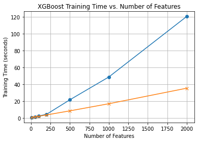
In all experiments, we observer a linear relationship between number of features and model training time.

Figure 1. Training Time as a function of Number of Features

This linear relationship holds for experiments done using CPU and GPU. Notably, GPU is observed to be two times as fast as CPU training on same datasets. However, experiments on CPU with feature sizes greater than 5000 did not complete. This suggests the additional cost of GPU relative to CPU is not worth the $0.50 / hour investment in the Lambda A10 for small datasets but GPUs are critical for training on larger data.

Figure 2. Training Time vs Number of Features on CPU & GPU

Limitations and Further Research

The experiments were limited to relatively small datasets and were time consuming given the constraints on GPU availability in Lambda cloud. Looking ahead, experiments to understand the marginal performance improvements based on GPU type are interesting but may not be possible to run using Lambda. Ideally, experiments with large GPUs such as A100 and H100 would offer more breadth to this research.

In the next post, we will explore the sensitivity of model training time to various xgboost hyperparameters: tree depth, learning rate, subsample and column sample while holding the other hyperparameters constant.

Conclusion

Throughout our exploration into the dynamics of training time with XGBoost regression, a clear linear relationship has emerged between the number of features and the time it takes to train our models. This underscores the importance of being mindful of feature selection and dimensionality, especially when working with large datasets or under time constraints.

Furthermore, our experiments have unveiled a notable distinction in training times between CPU and GPU. Specifically, leveraging GPU for training has consistently halved our model's training time compared to using a CPU. This 2x speed-up accentuates the growing significance of GPU-accelerated machine learning, offering a compelling case for investing in GPU resources, especially for data-intensive tasks.

As machine learning practitioners, these insights arm us with valuable knowledge, enabling more informed decisions in model development and resource allocation. As XGBoost continues to be a staple in the data scientist's toolkit, understanding its performance intricacies becomes ever more crucial.

References

XGBoost: A scalable tree boosting system

---